Understanding FlashAttention

Attention layers are notoriously memory-intensive. Their memory requirements grow quadratically with sequence length and as such, they consume memory far faster than they use compute, which is why training large transformers can often have you running out of memory. FlashAttention [1] offers one of the most elegant responses to this problem: it rethinks how attention is computed at the hardware level to dramatically cut memory overhead. Subsequent improvements in FlashAttention-2 [2] and FlashAttention-3 [3] further optimized the algorithm for modern GPU architectures, making it the perfect project for me to work through as a way to explore GPU programming in practice.

As a quick recap, the scaled dot-product attention for queries , keys , and values is:

Here, produces an attention matrix, which is then normalised with softmax before multiplying by . Note that is the sequence length and is the attention head dimension.

GPU execution model

To understand FlashAttention, it helps to first understand how GPUs execute code and organise memory. Modern GPUs are designed around a hierarchy of parallelism and memory that shapes how we write efficient kernels.

Threads, warps and blocks

A thread is the smallest unit of execution on a GPU. It executes a sequence of instructions such as additions, multiplications, memory loads and control flow. GPUs execute threads in groups called warps. A warp contains 32 threads¹ that execute the same instruction at the same time, but on different data (Single Instruction, Multiple Threads or SIMT). This is a hardware constraint: the GPU's warp scheduler physically issues one instruction to 32 threads at a time, keeping all threads in a warp synchronized on the same instruction at each clock cycle.

While warps are how threads are grouped together at a hardware-level, you typically define blocks to group threads at the software-level (sometimes called a Cooperative Thread Array or CTA in CUDA terminology). When you launch a kernel with a block size of 256 threads, you're creating 8 warps that will be scheduled together. Threads within a block can cooperate through shared memory, which is a key aspect to consider to minimise reads/writes when writing kernels.

Why this two-level abstraction? Warps give the hardware predictable, efficient SIMT execution, while blocks give programmers a flexible unit for organising work and memory sharing. A block can contain 1 to 32 warps: so up to 1024 threads on modern GPUs.

Warp schedulers are grouped together into Streaming Multiprocessors (SMs), which are self-contained compute units with their own warp schedulers, register file, and shared memory. Modern GPUs such as H100/B200 have over 100 SMs per chip, and each SM contains four warp schedulers that can issue instructions from four different warps concurrently. This hides latency: while one warp waits for memory, others can compute. When a thread block launches, it's assigned to an SM and stays there until completion. All its warps share that SM's register file and SRAM.

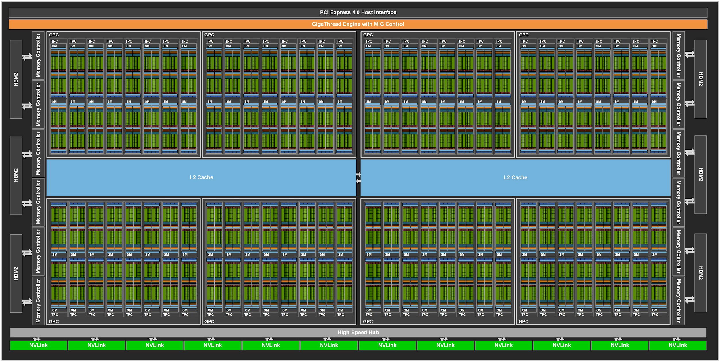GPU grid layout showing HBM on the sides (off-chip), multiple SMs on-chip (in green) with shared L2 cache (in blue). Each SM has its own warp schedulers, SRAM and register file.

Memory hierarchy

The GPU memory hierarchy reflects a tradeoff between speed and capacity:

• High Bandwidth Memory (HBM): slowest, largest (10s to 100s of GB), off-chip
• L2 cache: medium speed, moderate size (10s to 100s of MB), shared across all SMs
• Shared memory (SRAM): fast, small (100s of KB), shared within a thread block
• Registers: fastest (20x faster than SRAM), smallest, private to each thread

Fast kernels maximize reuse at each level: keep hot data in registers, stage intermediates in shared memory, and touch HBM as little as possible. The latency gap between SRAM and HBM is roughly 20×, which is why FlashAttention's core insight of keeping attention computation on-chip matters so much².

Standard attention kernels compute and store the entire attention matrix () in HBM, then fetch it again for softmax and for the multiplication with . This is what makes them memory-bound and consequently very slow as the matrices get large.

How does FlashAttention solve this?

FlashAttention reduces memory overhead through three ideas: tiling, online softmax, and kernel fusion.

Tiling

Tiling breaks a matrix into smaller blocks that fit in fast on-chip memory or SRAM, and the results of these block multiplications are accumulated to form the output matrix. It lets each block be reused multiple times while it stays in on-chip memory, reducing how often we need to go back to HBM. This idea isn't unique to FlashAttention, every GEMM (General Matrix Multiply) kernel relies on tiling, since large matrices could never fit on-chip at once. What FlashAttention does differently is to carry out all the computations required for attention on a tile before it ever leaves on-chip memory. By doing so, it avoids materializing the full matrix in HBM.

Tiling involves breaking a matrix into smaller blocks, computing their product and then accumulating the results.

Online softmax

While tiling breaks matrices into smaller blocks along both dimensions, softmax normalisation happens across entire rows (the full sequence dimension ). To normalize properly, we need the maximum value across all elements in a row, but our tiles only give us partial segments.

Online softmax solves this by tracking running statistics as we process tiles³. For each tile , we update the running maximum and sum :

The rescaling factor adjusts the previous sum when we find a new maximum, ensuring the normalisation base stays consistent. Note that we subtract the maximum () to prevent overflow when exponentiating large values.

This approach computes correct softmax probabilities without materializing the full attention matrix, enabling kernel fusion while maintaining mathematical correctness.

Calculating softmax in an online manner involves keeping track of the running max and sum and adjusting the results as each tile in the row gets processed.

Kernel fusion

In standard GPU kernels, computing , applying softmax, and multiplying by each run as separate kernels that read from and write to HBM. Intermediate results like the attention scores make multiple round-trips through memory.

Kernel fusion combines these into a single kernel. For each output row, FlashAttention processes tiles sequentially in SRAM: load and tiles, compute scores, update running statistics for the online softmax, rescale the partial output, multiply by , and accumulate. Only after all tiles in the row are processed does it write the final result to HBM.

Fusion + tiling avoid materializing in HBM, reducing HBM I/O for attention from quadratic in to linear in (for fixed ). This shifts the kernel toward being bandwidth-efficient and often compute-bound at practical sizes. See Horace He's blog post [4] for a great explanation with visual aids to understand kernel fusion more broadly.

Implementation in Triton

Understanding the ideas above conceptually is important, but implementing them in practice requires a different mental model given you’re writing code that maps directly to hardware threads. That means you have to reason explicitly about how data is laid out in memory, how to load it efficiently, and how to break the workload into manageable pieces that fit into registers and shared memory.

I'll use the Triton implementation here [5] as reference, and walk through some key ideas that underlie how the forward pass is structured. Rather than going line-by-line through the kernel, I'll focus on how the kernel maps the various algorithmic concepts discussed above to a concrete layout over GPU threads.

Working with batched inputs

Attention layers typically expect inputs of shape [B, H, N, d], where is the batch size, is the number of attention heads, is the sequence length, and is the head dimension. So for each query token, in a given sequence, in a given head, in a given batch, we want to compute an attention-weighted sum of the value vectors across the sequence.

The total number of such computations is , and each one produces a vector of size . This gives us an output tensor of the same shape: [B, H, N, d].

The input tensor has shape where each sequence position in each attention head in each batch contains a -dimensional embedding vector.

The Triton kernel flattens the [B, H] dimensions into a single dimension: . This is a practical move to simplify indexing. Triton assumes a 2D launch grid: so you typically use program_id(0) to index over rows (e.g., different tiles of the sequence), and program_id(1) to index over columns (e.g., different heads)⁴. Flattening [B, H] into a single dimension lets us fit the workload cleanly into this model and avoid additional complexity when mapping from thread IDs to tensor positions. Each program instance (i.e., thread block) can now operate on a single head in a single sequence without needing to manage nested loops over batch and head indices.

Visualising the algorithm

To make the kernel's flow concrete, let's walk through the forward pass of the algorithm below using a toy example where , , , and . This gives us full matrices of (concatenating both heads), with each per-head matrix being . Let's define the tile size in the row dimension, BLOCK_M, to be 4, meaning rows of will be loaded in blocks of 4. Similarly, let's define the tile size for and , BLOCK_N, to also be 4, meaning and are also loaded in blocks of 4⁵.

The visualization below is interactive: click on any cell in the grid to step through that program's forward pass and see how it loads tiles, updates running statistics, and produces its output.

Grid layout

The forward kernel _attn_fwd launches a 2D grid where each thread block (CTA) computes one tile of the output (note that q refers to the query matrix and N_CTX refers to the sequence length ):

// grid = (ceil(N_CTX, BLOCK_M), B*H, 1)
grid = (triton.cdiv(q.shape[2], META["BLOCK_M"]), q.shape[0]*q.shape[1], 1)

In our example, this produces a grid of shape i.e. 2 tiles along the sequence dimension and 8 flattened batch-head combinations (since ). The visualization above shows this as a grid where:

• program_id(0): vertical axis, labeled start_m, indexes which row block of the sequence we're processing
• program_id(1): horizontal axis, labeled off_hz, indexes which batch-head combination we're working on

Each program instance is responsible for computing a small [BLOCK_M, HEAD_DIM] tile of the output. Inside _attn_fwd, each program retrieves its coordinates and computes which batch and head it's responsible for:

start_m = tl.program_id(0)       # Which row block: 0 or 1
off_hz = tl.program_id(1)        # Which flattened batch-head index: 0 to 7
off_z = off_hz // H              # Batch index via floored division
off_h = off_hz % H               # Head index via modulo

Since is the outer dimension and is the inner dimension in the flattened layout, we determine the batch index by taking the floored division with the number of heads (off_z = off_hz // H) and the head index by taking the modulo with the number of heads (off_h = off_hz % H).

To walk through a concrete example, let's trace program 11. In the visualization grid at position , this corresponds to start_m = 1 and off_hz = 3, giving us off_z = 3 // 2 = 1 (batch 1) and off_h = 3 % 2 = 1 (head 1). Since start_m = 1 corresponds to the lower row-block or tile, program 11 computes rows 4-7 of the output for batch 1, head 1.

Pointer arithmetic and memory layout

A mental model to reason about indexing: imagine the matrices for each batch-head pair stacked vertically. With 4 batches and 2 heads, we have 8 separate matrices stacked into a conceptual tensor. In other words, we have 8 matrices stacked, each 8 rows in length, giving us a grid of 64 rows × 4 columns (head dimension). The offset_y variable determines the batch-head index by computing how many rows we need to skip: each batch has N_CTX * H elements and each head has N_CTX elements. Then qo_offset_y uses start_m to determine whether we're computing the top 4 rows (upper tile) or bottom 4 rows (lower tile) of that head.

offset_y = off_z * (N_CTX * H) + off_h * N_CTX
qo_offset_y = offset_y + start_m * BLOCK_M
offs_m = start_m * BLOCK_M + tl.arange(0, BLOCK_M)
offs_n = tl.arange(0, BLOCK_N)

For program 11, plugging in the values:

offset_y = 1 * (8 * 2) + 1 * 8 = 16 + 8 = 24
qo_offset_y = 24 + 1 * 4 = 28
offs_m = 4 + [0, 1, 2, 3] = [4, 5, 6, 7]
offs_n = [0, 1, 2, 3]

Here, offset_y = 24 points to the start of head 1 in batch 1 within the stacked tensor, and qo_offset_y = 28 points to the specific 4-row tile we're computing (rows 28-31 in the global layout, corresponding to rows 4-7 within this head). The array offs_m contains the global row indices within the head, while offs_n contains column offsets for indexing within tiles.

Outer loop: loading and initialization

Before entering the inner loop that streams tiles, _attn_fwd loads the tile into SRAM where it remains throughout⁶:

q = desc_q.load([qo_offset_y, 0])  # Shape: [BLOCK_M, HEAD_DIM] = [4, 4]

The kernel also initializes online softmax accumulators. The accumulator acc stores the running sum of softmax-weighted value vectors i.e., the partial output for this output tile.

m_i = tl.zeros([BLOCK_M], dtype=tl.float32)-float("inf") # [4] row-wise max
l_i = tl.zeros([BLOCK_M], dtype=tl.float32)+1.0          # [4] row-wise sum
acc = tl.zeros([BLOCK_M, HEAD_DIM], dtype=tl.float32)    # [4,4] accumulate

For causal attention, the kernel splits the computation into two stages handled by calling the inner function _attn_fwd_inner twice:

1. Stage 1 (off-band): processes tiles strictly to the left of the diagonal block
2. Stage 2 (on-band): processes the diagonal block itself with causal masking

For program 11, stage 1 processes columns 0-3 (off-band) and stage 2 processes columns 4-7 (the diagonal tile).

Inner loop: streaming tiles

Inside _attn_fwd_inner, the loop range is determined by the stage:

if STAGE == 1:  # Off-band tiles
    lo, hi = 0, start_m * BLOCK_M
elif STAGE == 2:  # On-band diagonal tile
    lo, hi = start_m * BLOCK_M, (start_m + 1) * BLOCK_M

For program 11 in stage 1, this gives lo = 0, hi = 4; in stage 2, lo = 4, hi = 8.

The inner loop streams through tiles, computing attention scores and updating the accumulator. For each tile, the kernel performs the following main operations⁷:

for start_n in tl.range(lo, hi, BLOCK_N):
    # Load K tile and compute QK^T scores
    k = desc_k.load([offsetk_y, 0]).T
    qk = tl.dot(q, k) * qk_scale
    
    # Apply causal mask on diagonal tile
    if STAGE == 2:
        mask = offs_m[:, None] >= (start_n + offs_n[None, :])
        qk = tl.where(mask, qk, -1.0e6)
    
    # Update running max and compute probabilities
    m_ij = tl.maximum(m_i, tl.max(qk, 1))
    p = tl.math.exp2(qk - m_ij[:, None])
    
    # Rescale previous accumulator and add new contribution
    alpha = tl.math.exp2(m_i - m_ij)
    acc = acc * alpha[:, None]
    v = desc_v.load([offsetv_y, 0])
    acc = tl.dot(p, v, acc)
    
    # Update running statistics
    l_i = l_i * alpha + tl.sum(p, 1)
    m_i = m_ij

For program 11 during stage 1 (start_n = 0), the kernel loads K[0:4, :] (transposed to [4, 4]), computes to get a score matrix, updates the running maximum m_ij and sum l_ij, applies the exponential to get probabilities p, computes the correction factor , loads V[0:4, :], and accumulates into acc after rescaling by .

During stage 2 (start_n = 4), the causal mask is applied. For rows [4, 5, 6, 7] and columns [4, 5, 6, 7], this produces a lower-triangular mask:

[[1, 0, 0, 0],   # Row 4 can only attend to col 4
 [1, 1, 0, 0],   # Row 5 can attend to cols 4-5
 [1, 1, 1, 0],   # Row 6 can attend to cols 4-6
 [1, 1, 1, 1]]   # Row 7 can attend to all cols 4-7

The mask suppresses future positions by adding to those attention scores before the softmax. Mathematically, the loop implements the online softmax recurrence:

The rescaling factor ensures correctness when the running maximum changes: when a new tile reveals a larger attention score, the algorithm retroactively adjusts the accumulator to maintain proper normalisation.

Epilogue: final normalisation

After processing all tiles, _attn_fwd performs final normalisation and writes the output⁸:

m_i += tl.math.log2(l_i)
acc = acc / l_i[:, None]
desc_o.store([qo_offset_y, 0], acc.to(dtype))

For program 11, this writes the final output tile to rows 28-31 of the flattened tensor (rows 4-7 of batch 1, head 1). Each program writes its output tile exactly once after all computations complete. The tile, tiles, and accumulator all remain in SRAM throughout, only the final result is written back to HBM. This "write-once" property, combined with tiling and online softmax, reduces HBM traffic from to and makes the kernel bandwidth-efficient.

The visualization mirrors this execution: when you select a grid cell, the corresponding rows highlight, then tiles pulse as the inner loop advances (off-band first, then the masked on-band tile), the causal mask overlay appears only during the diagonal iteration, the running scalars m_i and l_i update in the side panel, and finally the output rows flash when written to HBM.

Closing thoughts

Visualizing how FlashAttention maps to GPU hardware finally made the algorithm click for me. I hope the walkthrough and interactive animations help you build the same intuition.

The reference implementation used in this post is based on FlashAttention-2. Several important aspects remain unexplored: the kernel we examined supports FP8 computation for newer GPU architectures but we focused on the FP16 path for clarity; Hopper and Blackwell GPUs introduce hardware features like the Tensor Memory Accelerator that enable new optimizations; and FlashAttention-3 layers on additional techniques like warp specialization to overlap GEMM and softmax operations, asynchronous pipelining to hide memory latency, and careful block quantization for low-precision arithmetic. These are all natural next steps for anyone looking to push performance further.

More broadly, FlashAttention exemplifies a way of thinking about GPU kernels: identify the memory bottleneck, restructure the algorithm to maximize on-chip reuse, and map the computation carefully to hardware primitives. These principles extend well beyond attention: any memory-bound operation can benefit from similar ideas.

Footnotes

1. The 32-thread warp size is an NVIDIA-specific implementation detail. AMD GPUs use 64-thread wavefronts, though the SIMT execution model is conceptually similar. ↩

2. On an H100, SRAM has around 20-30 cycle latency while HBM can take 300-400 cycles. ↩

3. The online softmax technique predates FlashAttention and appears in earlier work on streaming algorithms. FlashAttention's contribution is applying it specifically to the attention mechanism with careful algorithmic and implementation co-design. ↩

4. Triton uses the term "program" to refer to a single instance of a kernel running on a tile of data, effectively one thread block. So program_id(0) and program_id(1) index which tile a program is working on. ↩

5. In practice, BLOCK_M and BLOCK_N are not chosen manually but tuned by running experiments. Triton also provides an autotuner for this. The choice is driven by how large of a tile can fit in SRAM and registers feasibly, typically ranging from 64 to 128 for realistic matrix sizes. ↩

6. Note that Triton assumes a row-major layout by default, so desc_q.load([i, j]) accesses row i and column j. ↩

7. The kernel uses exp2 (base-2 exponential) instead of natural exponential because modern GPUs have dedicated hardware instructions for exp2, making it faster. The algorithm maintains all statistics in log2 space and converts back during the final normalisation. ↩

8. The value m_i is stored to HBM after adding log2(l_i) for use in the backward pass, though we don't cover gradient computation in this post. ↩

References

- Dao, T., Fu, D. Y., Ermon, S., Rudra, A., & Ré, C. (2022). FlashAttention: Fast and Memory-Efficient Exact Attention with IO-Awareness. Advances in Neural Information Processing Systems, 35, 16344-16359.
- Dao, T. (2023). FlashAttention-2: Faster Attention with Better Parallelism and Work Partitioning. arXiv preprint arXiv:2307.08691.
- Shah, J., Bikshandi, G., Zhang, Y., Thakkar, V., Ramani, P., & Dao, T. (2024). FlashAttention-3: Fast and Accurate Attention with Asynchrony and Low-precision. arXiv preprint arXiv:2407.08608.
- He, H. (2022). Making Deep Learning Go Brrrr From First Principles. https://horace.io/brrr_intro.html
- Triton Language Documentation. (2024). Fused Attention Tutorial. https://triton-lang.org/main/getting-started/tutorials/06-fused-attention.html